Imbalance mapping analysis
Let’s get down to it! This module is relatively easy to use, but the explanation are slightly more complex.
Practice data
As always, sihnpy comes with data from the PREVENT-AD to be used as practice. In this case, structural MRI data, preprocessed with FreeSurfer is provided (see the PREVENT-AD preprocessing documentation for more info).
Imbalance mapping
1. Preparing the data
Imbalance mapping only requires:
A
pandas.DataFramewhereThe index is the participants’ IDs
The columns contain the variables you want to run the imbalance mapping on (e.g., thickness/volume).
If you already have your data, you can skip ahead to the next section.
Loading the data is super easy:
from sihnpy.datasets import pad_imb_input

volume_data, thickness_data, aseg_data = pad_imb_input()
thickness_data
| session | run | ctx_lh_bankssts_thickness | ctx_lh_caudalanteriorcingulate_thickness | ctx_lh_caudalmiddlefrontal_thickness | ctx_lh_cuneus_thickness | ctx_lh_entorhinal_thickness | ctx_lh_fusiform_thickness | ctx_lh_inferiorparietal_thickness | ctx_lh_inferiortemporal_thickness | ... | ctx_rh_rostralanteriorcingulate_thickness | ctx_rh_rostralmiddlefrontal_thickness | ctx_rh_superiorfrontal_thickness | ctx_rh_superiorparietal_thickness | ctx_rh_superiortemporal_thickness | ctx_rh_supramarginal_thickness | ctx_rh_frontalpole_thickness | ctx_rh_temporalpole_thickness | ctx_rh_transversetemporal_thickness | ctx_rh_insula_thickness | |
|---|---|---|---|---|---|---|---|---|---|---|---|---|---|---|---|---|---|---|---|---|---|
| participant_id | |||||||||||||||||||||
| sub-1000173 | ses-FU12 | run-001 | 2.153 | 2.334 | 2.451 | 1.767 | 3.202 | 2.452 | 2.161 | 2.515 | ... | 2.387 | 2.221 | 2.424 | 2.092 | 2.487 | 2.357 | 2.403 | 3.432 | 2.175 | 2.758 |
| sub-1002928 | ses-BL00 | run-001 | 2.462 | 2.403 | 2.449 | 1.735 | 3.316 | 2.664 | 2.253 | 2.586 | ... | 2.577 | 2.043 | 2.492 | 2.025 | 2.609 | 2.402 | 2.521 | 3.469 | 2.418 | 2.887 |
| sub-1004359 | ses-BL00 | run-001 | 2.246 | 2.276 | 2.346 | 1.815 | 3.332 | 2.728 | 2.388 | 2.620 | ... | 2.776 | 2.327 | 2.515 | 2.157 | 2.733 | 2.437 | 3.009 | 3.710 | 2.276 | 2.918 |
| sub-1004359 | ses-FU12 | run-001 | 2.238 | 2.339 | 2.349 | 1.827 | 3.449 | 2.674 | 2.403 | 2.610 | ... | 2.827 | 2.430 | 2.551 | 2.112 | 2.719 | 2.438 | 2.778 | 3.698 | 2.342 | 2.938 |
| sub-1016072 | ses-BL00 | run-001 | 2.213 | 2.544 | 2.327 | 1.662 | 3.310 | 2.580 | 2.295 | 2.603 | ... | 2.440 | 2.224 | 2.435 | 2.084 | 2.583 | 2.461 | 2.710 | 3.735 | 2.302 | 2.810 |
| ... | ... | ... | ... | ... | ... | ... | ... | ... | ... | ... | ... | ... | ... | ... | ... | ... | ... | ... | ... | ... | ... |
| sub-9930257 | ses-BL00 | run-001 | 2.435 | 2.476 | 2.511 | 1.893 | 2.903 | 2.557 | 2.397 | 2.645 | ... | 2.825 | 2.249 | 2.656 | 2.183 | 2.729 | 2.474 | 2.620 | 3.617 | 2.629 | 2.890 |
| sub-9931234 | ses-BL00 | run-001 | 2.461 | 2.166 | 2.526 | 1.755 | 3.143 | 2.618 | 2.383 | 2.918 | ... | 2.606 | 2.252 | 2.500 | 2.200 | 2.710 | 2.466 | 2.496 | 3.257 | 2.497 | 2.879 |
| sub-9931234 | ses-FU12 | run-001 | 2.403 | 2.194 | 2.536 | 1.756 | 3.216 | 2.594 | 2.345 | 2.837 | ... | 2.660 | 2.256 | 2.518 | 2.213 | 2.750 | 2.435 | 2.632 | 3.380 | 2.566 | 2.742 |
| sub-9939055 | ses-BL00 | run-001 | 2.332 | 2.743 | 2.460 | 1.648 | 3.010 | 2.609 | 2.387 | 2.610 | ... | 2.641 | 2.152 | 2.442 | 2.159 | 2.759 | 2.473 | 2.557 | 3.901 | 2.263 | 2.916 |
| sub-9939055 | ses-FU12 | run-001 | 2.312 | 2.611 | 2.456 | 1.622 | 2.960 | 2.583 | 2.324 | 2.610 | ... | 2.574 | 2.134 | 2.460 | 2.147 | 2.695 | 2.478 | 2.559 | 3.814 | 2.317 | 3.057 |
541 rows × 70 columns
As I mentioned in the introduction, sihnpy assumes that the data has a single row for each participant. However, to give you more practice opportunities, sihnpy data for this module comes with two visits: BL00 and FU12. For now, we will restrict the data to only the baseline visits and drop the “session” and “run” variables as they aren’t needed.
thickness_data_final = thickness_data[thickness_data['session'] == 'ses-BL00'].drop(labels=['session', 'run'], axis=1)
thickness_data_final #We get the 68 columns of data needed
| ctx_lh_bankssts_thickness | ctx_lh_caudalanteriorcingulate_thickness | ctx_lh_caudalmiddlefrontal_thickness | ctx_lh_cuneus_thickness | ctx_lh_entorhinal_thickness | ctx_lh_fusiform_thickness | ctx_lh_inferiorparietal_thickness | ctx_lh_inferiortemporal_thickness | ctx_lh_isthmuscingulate_thickness | ctx_lh_lateraloccipital_thickness | ... | ctx_rh_rostralanteriorcingulate_thickness | ctx_rh_rostralmiddlefrontal_thickness | ctx_rh_superiorfrontal_thickness | ctx_rh_superiorparietal_thickness | ctx_rh_superiortemporal_thickness | ctx_rh_supramarginal_thickness | ctx_rh_frontalpole_thickness | ctx_rh_temporalpole_thickness | ctx_rh_transversetemporal_thickness | ctx_rh_insula_thickness | |
|---|---|---|---|---|---|---|---|---|---|---|---|---|---|---|---|---|---|---|---|---|---|
| participant_id | |||||||||||||||||||||
| sub-1002928 | 2.462 | 2.403 | 2.449 | 1.735 | 3.316 | 2.664 | 2.253 | 2.586 | 2.130 | 2.116 | ... | 2.577 | 2.043 | 2.492 | 2.025 | 2.609 | 2.402 | 2.521 | 3.469 | 2.418 | 2.887 |
| sub-1004359 | 2.246 | 2.276 | 2.346 | 1.815 | 3.332 | 2.728 | 2.388 | 2.620 | 2.258 | 2.150 | ... | 2.776 | 2.327 | 2.515 | 2.157 | 2.733 | 2.437 | 3.009 | 3.710 | 2.276 | 2.918 |
| sub-1016072 | 2.213 | 2.544 | 2.327 | 1.662 | 3.310 | 2.580 | 2.295 | 2.603 | 1.986 | 2.035 | ... | 2.440 | 2.224 | 2.435 | 2.084 | 2.583 | 2.461 | 2.710 | 3.735 | 2.302 | 2.810 |
| sub-1031654 | 2.455 | 2.340 | 2.355 | 1.842 | 3.381 | 2.833 | 2.290 | 2.653 | 2.324 | 2.194 | ... | 2.643 | 2.307 | 2.628 | 2.052 | 2.692 | 2.441 | 3.035 | 3.873 | 2.224 | 3.056 |
| sub-1072774 | 2.403 | 2.480 | 2.485 | 1.752 | 3.443 | 2.672 | 2.356 | 2.890 | 2.561 | 2.057 | ... | 2.760 | 2.247 | 2.593 | 2.147 | 2.577 | 2.451 | 2.315 | 3.758 | 2.195 | 3.140 |
| ... | ... | ... | ... | ... | ... | ... | ... | ... | ... | ... | ... | ... | ... | ... | ... | ... | ... | ... | ... | ... | ... |
| sub-9889544 | 2.438 | 2.438 | 2.441 | 1.838 | 3.306 | 2.613 | 2.315 | 2.682 | 2.169 | 2.218 | ... | 2.644 | 2.227 | 2.532 | 2.271 | 2.863 | 2.475 | 2.226 | 3.697 | 2.561 | 2.727 |
| sub-9909448 | 2.502 | 2.062 | 2.359 | 1.750 | 3.127 | 2.642 | 2.314 | 2.675 | 1.962 | 2.073 | ... | 2.524 | 2.311 | 2.508 | 2.043 | 2.664 | 2.384 | 2.477 | 3.666 | 2.634 | 2.769 |
| sub-9930257 | 2.435 | 2.476 | 2.511 | 1.893 | 2.903 | 2.557 | 2.397 | 2.645 | 2.280 | 2.080 | ... | 2.825 | 2.249 | 2.656 | 2.183 | 2.729 | 2.474 | 2.620 | 3.617 | 2.629 | 2.890 |
| sub-9931234 | 2.461 | 2.166 | 2.526 | 1.755 | 3.143 | 2.618 | 2.383 | 2.918 | 2.065 | 2.223 | ... | 2.606 | 2.252 | 2.500 | 2.200 | 2.710 | 2.466 | 2.496 | 3.257 | 2.497 | 2.879 |
| sub-9939055 | 2.332 | 2.743 | 2.460 | 1.648 | 3.010 | 2.609 | 2.387 | 2.610 | 2.095 | 2.096 | ... | 2.641 | 2.152 | 2.442 | 2.159 | 2.759 | 2.473 | 2.557 | 3.901 | 2.263 | 2.916 |
306 rows × 68 columns
2. Imbalance mapping
Ok now is the fun part: the imbalance mapping. The code behind is complex, but the application is simple. The function only requires two input:
A
pandas.DataFramewith the index as the participant IDs and the columns being the variables we want to map.The
typeof orthogonal distances we want to get.
The type of distances is simply whether we want absolute (abs) distances or signed (sign) distances from the regression slope. In the absolute version, we don’t care whether the fitted value is above or below the diagonal: we just want to know how far the value is. In the signed version, we want to know whether the fitted value was overestimated (i.e., above the regression line) or underestimated (i.e., below the regression line). Whether you want absolute or signed distances is really up to you. In the original article by Nadig et al. (2021)1, the absolute residuals were used. Here is the code to run it:
from sihnpy import imbalance_mapping as imb

residual_array = imb.imbalance_mapping(data=thickness_data_final, type='abs')
Computing region 1/68
Computing region 2/68
Computing region 3/68
Computing region 4/68
Computing region 5/68
Computing region 6/68
Computing region 7/68
Computing region 8/68
Computing region 9/68
Computing region 10/68
Computing region 11/68
Computing region 12/68
Computing region 13/68
Computing region 14/68
Computing region 15/68
Computing region 16/68
Computing region 17/68
Computing region 18/68
Computing region 19/68
Computing region 20/68
Computing region 21/68
Computing region 22/68
Computing region 23/68
Computing region 24/68
Computing region 25/68
Computing region 26/68
Computing region 27/68
Computing region 28/68
Computing region 29/68
Computing region 30/68
Computing region 31/68
Computing region 32/68
Computing region 33/68
Computing region 34/68
Computing region 35/68
Computing region 36/68
Computing region 37/68
Computing region 38/68
Computing region 39/68
Computing region 40/68
Computing region 41/68
Computing region 42/68
Computing region 43/68
Computing region 44/68
Computing region 45/68
Computing region 46/68
Computing region 47/68
Computing region 48/68
Computing region 49/68
Computing region 50/68
Computing region 51/68
Computing region 52/68
Computing region 53/68
Computing region 54/68
Computing region 55/68
Computing region 56/68
Computing region 57/68
Computing region 58/68
Computing region 59/68
Computing region 60/68
Computing region 61/68
Computing region 62/68
Computing region 63/68
Computing region 64/68
Computing region 65/68
Computing region 66/68
Computing region 67/68
Computing region 68/68
So, what did we do, and what did we get?
In this step, we do the equivalent of step B) and C) from Nadig et al. (2021)’s figure: we compute the structural covariance and extract the orthogonal distances for each participant. This is store in a massive 3D matrix (well… I guess it’s a rectangle at this point):
residual_array.shape
(68, 68, 306)
Here’s a simplified illustration of what it would look like if we illustrated this:

In this cube, each square matrix represent the orthogonal distances from the regression of the values of two regions for a single participant. The diagonal is removed (in the image it is whited out) as the correlation of the same column twice would give a perfect correlation.
While the shape of the image is much smaller than the actual matrix (68 regions X 68 regions X 306 participants), the principle is exactly the same.
Once this 3D matrix is calculated, we are already ready to compute our measures.
Warning: Using more than one predictor
In the current implementation of imbalance mapping–as well as the original implementation–the ODR is used assuming a single predictor. However, like any regression, the ODR can be used using multiple covariates. The implementation of the ODR function in sihnpy theoretically allows for that too as it was translated from pracma, which specifically accounts for that.
However, I haven’t tested this when developping sihnpy and the imbalance_mapping function does not allow for controlling for covariates yet. The function will consider each column in your dataframe as both outcome and predictor in their own turn, so it is extra important to only include brain data in the columns you feed to imbalance_mapping.
If you want to control for other variables in your analyses, my suggestion for now would be either to follow Nadig’s approach and regress out the covariates of each column of brain data before running it in imbalance_mapping OR run the imbalance_mapping and subsequently verify if the measures you get from module are associated with your covariates.
If you would like the imbalance mapping module to be able to include covariates feel free to request the feature by opening an issue.
3. Imbalance statistics
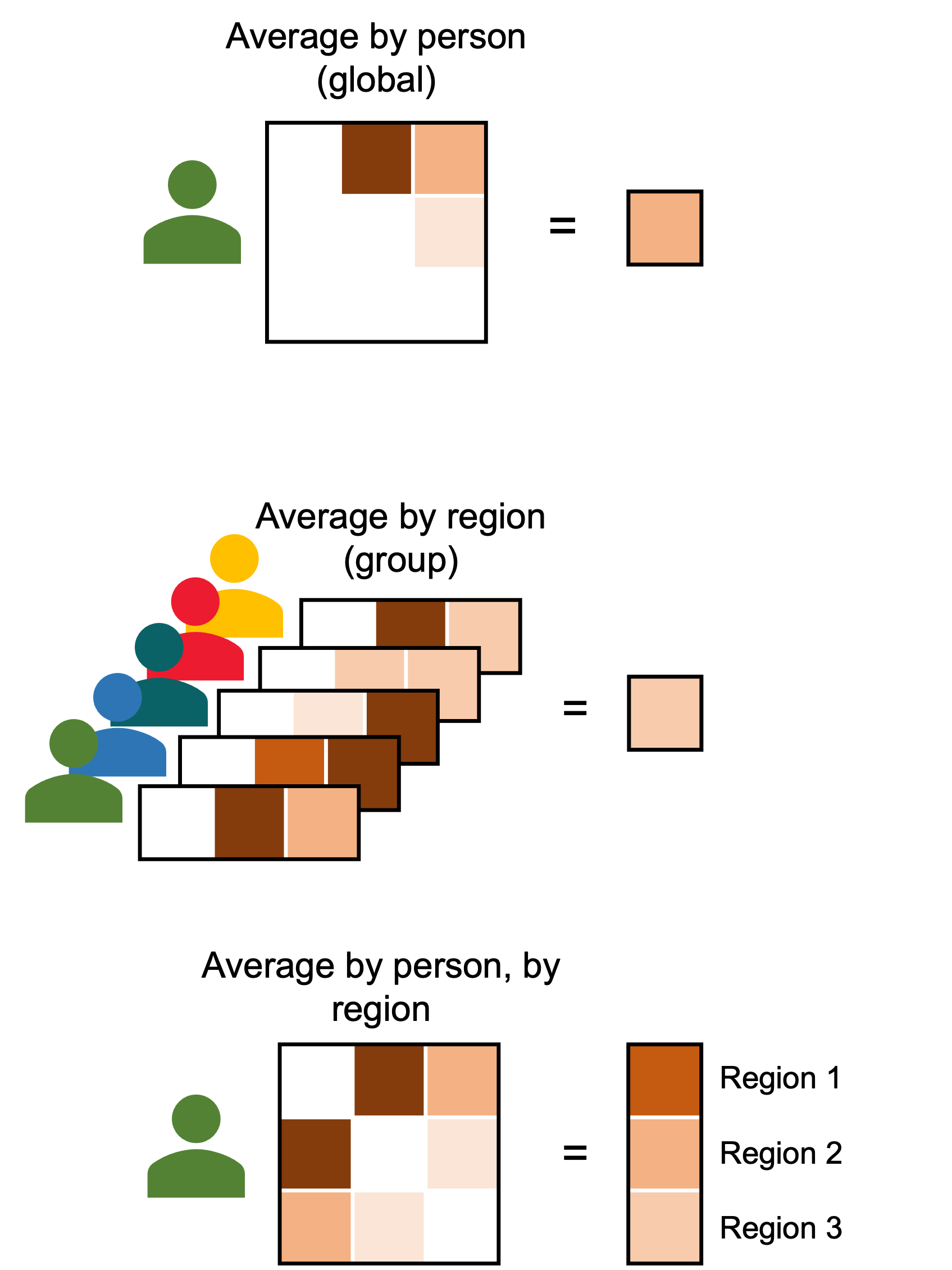
In the original code by Nadig et al. (2021)1 proposes two measures: computing an average imbalance by person (i.e., average imbalance across all edges) and an average imbalance by region at the group-level (i.e., how much imbalance does the entorhinal cortex show for example). sihnpy integrates both measures, but also outputs an average imbalance by person by region (i.e., how much imbalance on average the entorhinal cortex shows in person Y). Below is a quick illustration of these measures:
These measures in sihnpy can be calculated very easily with a single function taking two arguments:
The original
pandas.DataFrameused to compute the imbalance mapping (we use it to grab the participant IDs and the region names)The cube of orthogonal distances we computed in the previous step
avg_imb_by_region, avg_imb_by_person, avg_imb_by_pers_by_region = imb.imbalance_stats(data=thickness_data_final, residual_array=residual_array)
avg_imb_by_pers_by_region
| ctx_lh_bankssts_thickness | ctx_lh_caudalanteriorcingulate_thickness | ctx_lh_caudalmiddlefrontal_thickness | ctx_lh_cuneus_thickness | ctx_lh_entorhinal_thickness | ctx_lh_fusiform_thickness | ctx_lh_inferiorparietal_thickness | ctx_lh_inferiortemporal_thickness | ctx_lh_isthmuscingulate_thickness | ctx_lh_lateraloccipital_thickness | ... | ctx_rh_rostralanteriorcingulate_thickness | ctx_rh_rostralmiddlefrontal_thickness | ctx_rh_superiorfrontal_thickness | ctx_rh_superiorparietal_thickness | ctx_rh_superiortemporal_thickness | ctx_rh_supramarginal_thickness | ctx_rh_frontalpole_thickness | ctx_rh_temporalpole_thickness | ctx_rh_transversetemporal_thickness | ctx_rh_insula_thickness | |
|---|---|---|---|---|---|---|---|---|---|---|---|---|---|---|---|---|---|---|---|---|---|
| participant_id | |||||||||||||||||||||
| sub-1002928 | 0.050868 | 0.070757 | 0.045348 | 0.131103 | 0.090582 | 0.031317 | 0.051684 | 0.129795 | 0.064045 | 0.060393 | ... | 0.068125 | 0.135052 | 0.065608 | 0.109356 | 0.045579 | 0.079806 | 0.069990 | 0.066805 | 0.066181 | 0.055967 |
| sub-1004359 | 0.108628 | 0.077152 | 0.080876 | 0.046602 | 0.079860 | 0.047387 | 0.043844 | 0.062625 | 0.063184 | 0.030747 | ... | 0.084405 | 0.057178 | 0.032863 | 0.028792 | 0.048641 | 0.036213 | 0.106226 | 0.087844 | 0.076241 | 0.052139 |
| sub-1016072 | 0.153541 | 0.107828 | 0.115252 | 0.146310 | 0.103709 | 0.076043 | 0.052581 | 0.096220 | 0.122770 | 0.121347 | ... | 0.109038 | 0.055124 | 0.100050 | 0.076545 | 0.084167 | 0.045742 | 0.106502 | 0.111446 | 0.104460 | 0.073354 |
| sub-1031654 | 0.059193 | 0.076811 | 0.079381 | 0.051086 | 0.083903 | 0.122421 | 0.063430 | 0.054097 | 0.080342 | 0.043770 | ... | 0.074475 | 0.055412 | 0.086878 | 0.091662 | 0.046471 | 0.039275 | 0.108813 | 0.095604 | 0.096446 | 0.109220 |
| sub-1072774 | 0.042627 | 0.075648 | 0.045346 | 0.077476 | 0.082345 | 0.032254 | 0.027092 | 0.146982 | 0.140083 | 0.094995 | ... | 0.080289 | 0.039019 | 0.051833 | 0.029578 | 0.097529 | 0.030800 | 0.105583 | 0.080944 | 0.091024 | 0.153880 |
| ... | ... | ... | ... | ... | ... | ... | ... | ... | ... | ... | ... | ... | ... | ... | ... | ... | ... | ... | ... | ... | ... |
| sub-9889544 | 0.047168 | 0.063802 | 0.037739 | 0.045298 | 0.073720 | 0.063764 | 0.037288 | 0.041076 | 0.057354 | 0.052754 | ... | 0.067646 | 0.048609 | 0.030474 | 0.097550 | 0.132909 | 0.032159 | 0.100336 | 0.081138 | 0.083595 | 0.106776 |
| sub-9909448 | 0.065361 | 0.116467 | 0.081611 | 0.086068 | 0.089651 | 0.043559 | 0.036690 | 0.044671 | 0.114514 | 0.081760 | ... | 0.082605 | 0.052499 | 0.040859 | 0.095083 | 0.046149 | 0.076434 | 0.090830 | 0.089720 | 0.106595 | 0.079453 |
| sub-9930257 | 0.056596 | 0.089051 | 0.057623 | 0.055001 | 0.106769 | 0.101592 | 0.058074 | 0.063256 | 0.078726 | 0.079335 | ... | 0.112533 | 0.043268 | 0.098764 | 0.040644 | 0.056836 | 0.039443 | 0.092014 | 0.096737 | 0.110040 | 0.056424 |
| sub-9931234 | 0.050102 | 0.107396 | 0.058061 | 0.087155 | 0.090427 | 0.055866 | 0.046965 | 0.156671 | 0.083045 | 0.054264 | ... | 0.074458 | 0.037636 | 0.043781 | 0.048241 | 0.044734 | 0.033495 | 0.094016 | 0.108685 | 0.074805 | 0.050416 |
| sub-9939055 | 0.085146 | 0.112179 | 0.041061 | 0.163699 | 0.092641 | 0.058380 | 0.052383 | 0.088371 | 0.078373 | 0.073949 | ... | 0.074229 | 0.077621 | 0.098613 | 0.033443 | 0.071312 | 0.034188 | 0.082869 | 0.098912 | 0.085072 | 0.058322 |
306 rows × 68 columns
And that’s it! You have everything you need to run the analysis on your own.
Advanced topic: Subsetting specific regions for averaging
In some cases, you may want to check the average imbalance in specific, pre-defined networks for instance. For instance, let’s say you are investigating the imbalance mapping specifically in the temporal lobe. In such a case, you may be interested in computing the imbalance only in a specific set of regions. However, sihnpy doesn’t yet natively support this. Two options are offered to you in this case:
Either you restrict your data (i.e.,
thickness_data_final) to include only the columns you are interested in.You manipulate the
residual_arrayto select only the parts of the rectangle that interest you.
The first solution is probably easiest, but it will require you to recompute the imbalance mapping for every different set of regions you want which may get computationally expensive when running it on many regions and/or combinations of regions.
The second solution is more complicated to do and require good knowledge of a array slicing in Numpy. It can take some getting used to, particularly when working in 3D. However, in this method, you only need to compute imbalance mapping once, and then you just need to feed the different slices to imbalance_stats which is much less computationally expensive.
If there is enough interest, I will adapt a way to do this natively in sihnpy. Open an issue if you are interested!
Bonus: Here are a few examples of what you can plot once you have the imbalance data.
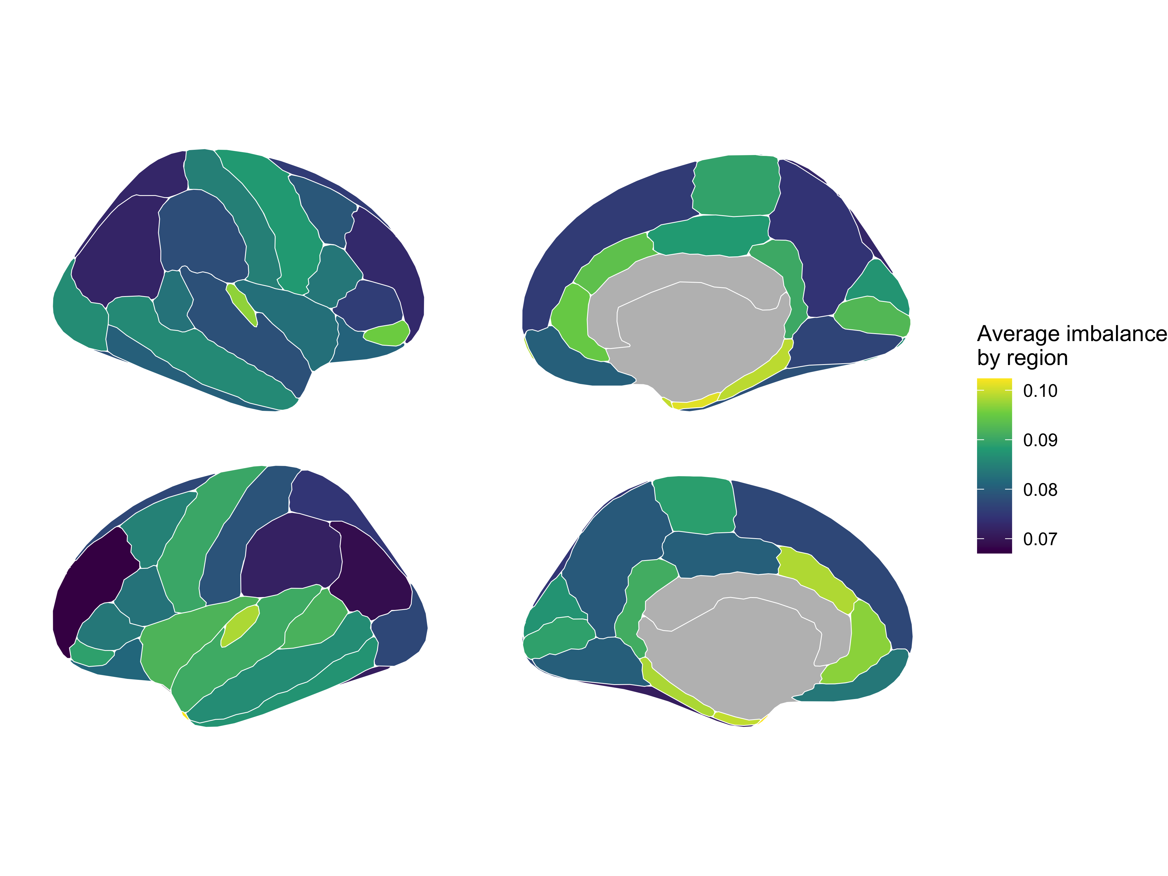
Average imbalance by region
This plot was done using the library ggseg in R. There is a version of ggseg in Python that recently came out, but I am not yet used to it.
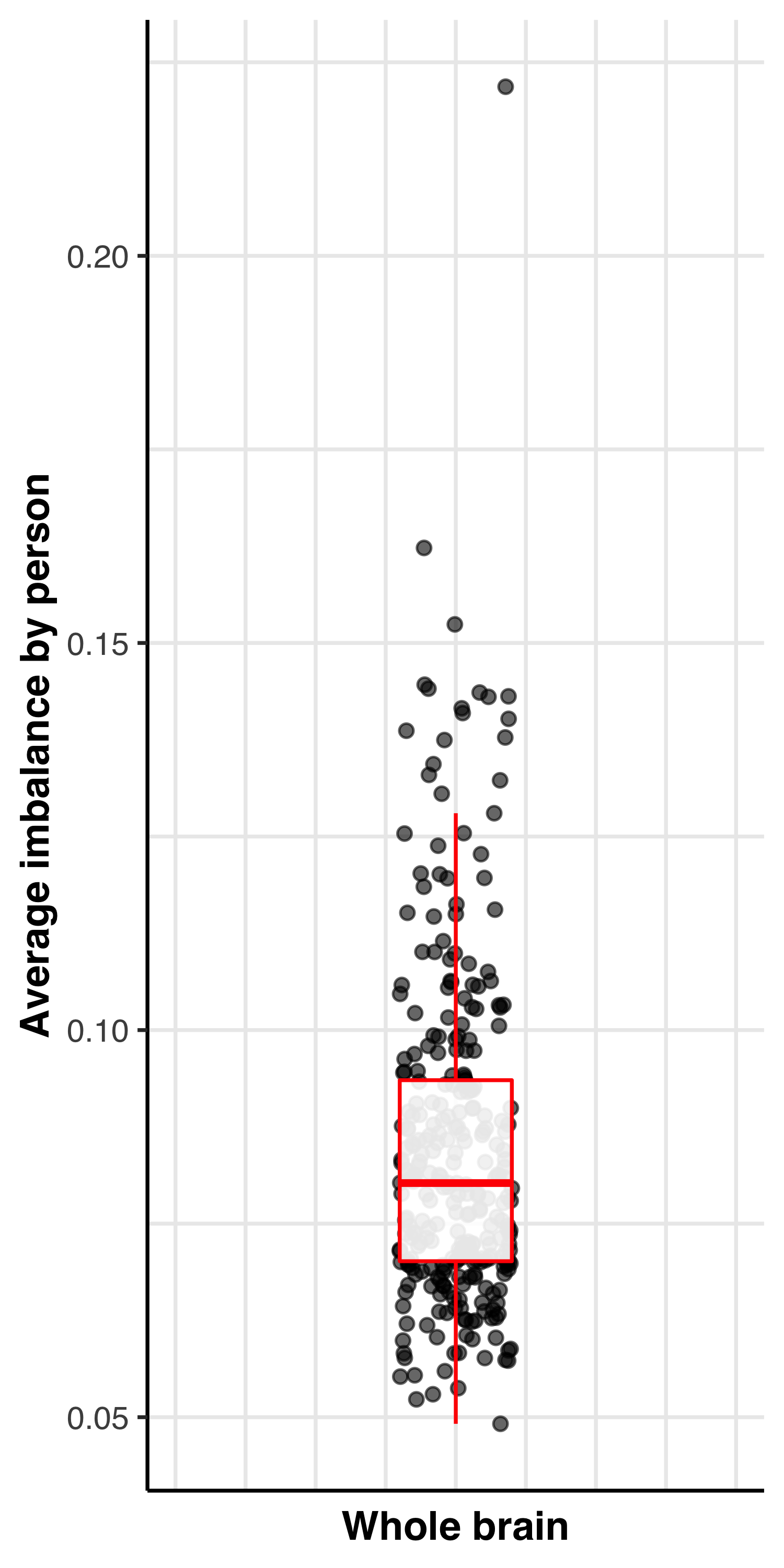
Average imbalance by person
This plot is the average imbalance of each participant across the whole brain. Plotted in R with ggplot2.
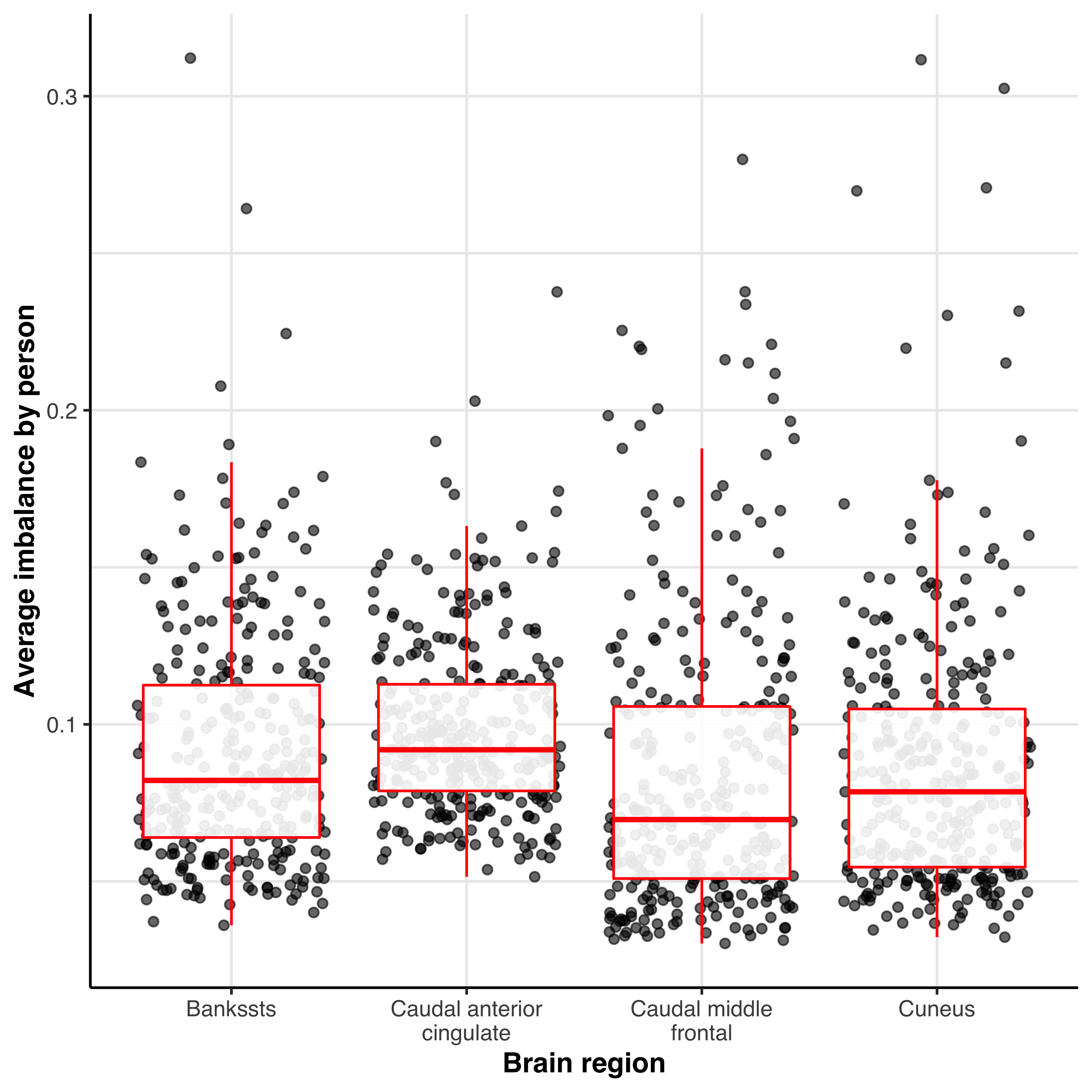
Average imbalance by person by region
Average imbalance in each cortical region for each participant. Only 4 regions are plotted for consiceness. Plotted in R with ggplot2.
4. Export
The next function needs a lot of arguments, but the goal is very simple: output the different measures computed during the imbalance mapping analysis. To output, simply follow the following command:
imb.export(data=thickness_data_final, residual_array=residual_array, output_path="/path/to/output", avg_imb_by_region=avg_imb_by_region, avg_imb_by_person=avg_imb_by_person, avg_imb_by_pers_by_region=avg_imb_by_pers_by_region, name='test', all=False)
The only choice the user has over is whether we should export the matrices of orthogonal distances for each participant. This could be useful for other analyses but will require a lot more space. By default, this is not output, but the user can choose to do so by switching False to True.
tl;dr
Too lazy to read everything? Or read everything and need a quick refresher? Here is the code in the order you need to make it work.
from sihnpy.datasets import pad_imb_input #For practice data
from sihnpy import imbalance_mapping as imb #Imbalance mapping functions

volume_data, thickness_data, aseg_data = pad_imb_input() #Import the practice data
#If the data has more than 1 row by participant, clean the data
thickness_data_final = thickness_data[thickness_data['session'] == 'ses-BL00'].drop(labels=['session', 'run'], axis=1)

#Imbalance mapping
residual_array = imb.imbalance_mapping(data=thickness_data_final, type='abs')
avg_imb_by_region, avg_imb_by_person, avg_imb_by_pers_by_region = imb.imbalance_stats(data=thickness_data_final, residual_array=residual_array)

#Export
imb.export(data=thickness_data_final, residual_array=residual_array, output_path="/path/to/output", avg_imb_by_region=avg_imb_by_region, avg_imb_by_person=avg_imb_by_person, avg_imb_by_pers_by_region=avg_imb_by_pers_by_region, name='test', all=False)
Appendix - Orthogonal Distance Regression (ODR)
Imbalance mapping in its original form1 leverages a special type of regression called Orthogonal Distance Regression (ODR) (also sometimes called total least square, or Denim regression). This is implemented by default in sihnpy’s function. However, sihnpy also exposes the function for users who would like to use it.
Warning
I should preface this section by saying that, while I have experience with principal component analysis (which is the basis of ODR in the form it is implemented), I am by no means a mathematician so some of the math involved go way over my head and the implementation involves some (or at lot) of trust in the original implementation. However, in my tests, results I got with sihnpy were entirely replicated using the original R library pracma as well as scipy’s ODR implementation which makes me more confident in its implementation here.
Rationale
When doing a traditional regression–which refers most of the time to an Ordinary Least Square (OLS) regression–we try to find the slope that minimizes the error between the outcome (Y) variable and the slope. The goal here is to obtain the best possible slope describing the relationship between predictor and outcome. However, OLS assumes that there are only measurement errors on the outcome variable, which can become problematic when using an OLS regression between a predictor and outcome that can both have measurement error.2
This is problematic specifically in our case. When we do structural covariance, we correlate the values in two brain regions, which may both have measurement error. So how do we resolve this?
Cue in ODR.
Instead of minimizing the distance between the outcome variable and the slope, ODR minimizes the distance perpendicular to the slope on both the predictor and outcome.2,3 This has the theoretical advantage of assuming that both the predictor and outcome have error2 which is an attractive option in our case. But how does one figure out the slope minimizing the orthogonal distance between the slope and the datapoints? I’m glad you asked. A relatively easy way of doing this is to leverage Principal Component Analysis (PCA).
In a PCA analysis, the goal is generally to create new variables that can summarize variables in a dataset but conserve as much variance as possible. This is so we can do what is called dimensionality reduction; we want to reduce the number of variables we need to use in our analyses but without losing important information (i.e. variance).[^Jolliffe_2016]
The PCA will always return the same number of components as the number of variables that are input to it. In our case, the first component represents the slope that minimizes the orthogonal distances and the second component is the error; i.e., the orthogonal distance. The software needs to do some mathematical gymnastics to extract both, but that is the general gyst of it.
Running ODR in sihnpy
In most cases, if you use sihnpy for imbalance mapping, you won’t really need to dive in to the use of ODR. However, if you are interested, the original implementation of ODR in the pracma library does output more information on the ODR. In sihnpy we really only extract the orthogonal distances, but you could also obtain the slope, intercept, etc.
Let’s do an example by selecting two columns from our thickness_data_final we used earlier. We’ll use ODR to associate the thickness of the caudal anterior cingulate in the left hemisphere to the thickness of the caudal middle frontal cortex in the left hemisphere.
subsample = thickness_data_final[['ctx_lh_caudalanteriorcingulate_thickness', 'ctx_lh_caudalmiddlefrontal_thickness']]
subsample
| ctx_lh_caudalanteriorcingulate_thickness | ctx_lh_caudalmiddlefrontal_thickness | |
|---|---|---|
| participant_id | ||
| sub-1002928 | 2.403 | 2.449 |
| sub-1004359 | 2.276 | 2.346 |
| sub-1016072 | 2.544 | 2.327 |
| sub-1031654 | 2.340 | 2.355 |
| sub-1072774 | 2.480 | 2.485 |
| ... | ... | ... |
| sub-9889544 | 2.438 | 2.441 |
| sub-9909448 | 2.062 | 2.359 |
| sub-9930257 | 2.476 | 2.511 |
| sub-9931234 | 2.166 | 2.526 |
| sub-9939055 | 2.743 | 2.460 |
306 rows × 2 columns
You can do an ODR by calling the function imb.odregression_single. It requires 3 things: the index of the dataframe (i.e., the participant IDs), the column to be used as “predictor” (i.e., x) and the column to be used as “outcome” (i.e., y).
individual_values, model_fit_data = imb.odregression_single(index=subsample.index, x=subsample['ctx_lh_caudalanteriorcingulate_thickness'].values, y=subsample['ctx_lh_caudalmiddlefrontal_thickness'])
We get two objects returned. Let’s take a look.
individual_values
| y_values | fitted_values | residuals | absolute_orthogonal_distances | signed_orthogonal_distances | |
|---|---|---|---|---|---|
| participant_id | |||||
| sub-1002928 | 2.449 | 2.451235 | -0.002235 | 0.002227 | -0.002227 |
| sub-1004359 | 2.346 | 2.440694 | -0.094694 | 0.094369 | -0.094369 |
| sub-1016072 | 2.327 | 2.462938 | -0.135938 | 0.135473 | -0.135473 |
| sub-1031654 | 2.355 | 2.446006 | -0.091006 | 0.090694 | -0.090694 |
| sub-1072774 | 2.485 | 2.457626 | 0.027374 | 0.027280 | 0.027280 |
| ... | ... | ... | ... | ... | ... |
| sub-9889544 | 2.441 | 2.454140 | -0.013140 | 0.013095 | -0.013095 |
| sub-9909448 | 2.359 | 2.422931 | -0.063931 | 0.063712 | -0.063712 |
| sub-9930257 | 2.511 | 2.457294 | 0.053706 | 0.053522 | 0.053522 |
| sub-9931234 | 2.526 | 2.431563 | 0.094437 | 0.094113 | 0.094113 |
| sub-9939055 | 2.460 | 2.479456 | -0.019456 | 0.019389 | -0.019389 |
306 rows × 5 columns
The individual_values object contains everything that is calculated on an individual level. It holds the original y value for each participant, the new fitted value output from the regression, the residuals (i.e., the distance between the fitted value and the slope on the Y-axis only) and the orthogonal distances. The residuals are signed and the orthogonal distances come in both signed and unsigned format (matching the code proposed by Nadig et al. (2021)1).
model_fit_data
| values | |
|---|---|
| slope | 2.251779 |
| intercept | 0.083003 |
| total_sum_of_squares | 3.180038 |
This dataframe outputs the slope, the intercept and the total sum of squares for the model.
You might notice that the residuals and the orthogonal distances are not very different. In the original paper by Nadig et al. (2021),1 the samples used included participants whose brain were still in development (i.e., children and teenagers). In these samples, the brain is still growing and structural covariance can give more differences in estimates when comparing OLS and ODR.
It also really depends on the variables you use in the regression, but most of the time with the PREVENT-AD data included in this package, there isn’t a lot of difference between using a traditional OLS regression or a ODR regression. See below the example from the two regions we just correlated:

In that example, the slope given by the OLS is: y = 2.307x + 0.060 In that example, the slope given by the ODR is: y = 2.252x + 0.083
Theoretically however, more so when the predictor and outcome have the same burden of error, this method should give more precise estimates.
References
Here are the references of this section:
- 1(1,2,3,4,5)
Nadig A, Seidlitz J, McDermott CL, Liu S, Bethlehem R, Moore TM, Mallard TT, Clasen LS, Blumenthal JD, Lalonde F, Gur RC, Gur RE, Bullmore ET, Satterthwaite TD, Raznahan A. Morphological integration of the human brain across adolescence and adulthood. Proc Natl Acad Sci U S A. 2021 Apr 6;118(14):e2023860118. doi: 10.1073/pnas.2023860118. PMID: 33811142; PMCID: PMC8040585.
- 2(1,2,3)
James R. Carr (2012) Orthogonal regression: a teaching perspective, International Journal of Mathematical Education in Science and Technology, 43:1, 134-143, DOI: 10.1080/0020739X.2011.573876
- 3
Pallavi, Joshi, S., Singh, D. et al. Comprehensive Review of Orthogonal Regression and Its Applications in Different Domains. Arch Computat Methods Eng 29, 4027–4047 (2022). doi: 10.1007/s11831-022-09728-5