Introduction to imbalance mapping

Welcome to the imbalance mapping module!

Note

This module is the only one in sihnpy that hasn’t been used in a publication I made. However, the code was tested against the original R code developped by Nadig et al. (2021)1. Feel free to report any issues or suggestions by opening an issue

Rationale

If you have read the documentation on the fingerprinting module, you might remember that in the fingerprinting analysis, we correlate the patterns of functional connectivity between individuals to determine how similar an individual is to themselves or to others. However, the way the analysis is set up requires two different sessions for each individuals. Instead, we could imagine that, rather than determining how similar an individual is to their cohort (i.e., others-identifiability), we could ask the question: how different is an individual to the rest of their cohort?

This was the question that Nadig et al. (2021)1 asked. In the original study, the goal was to determine how much deviation an individual displayed from developmental norms (i.e., population average). This is done by leveraging a technique called structural covariance. Structural covariance is a rich field that I won’t dive into here but the general idea is to correlate grey matter measures (volume, thickness, etc.) between two regions in a group of individuals. A stronger correlation between regions is thought to represent coordinated change in anatomy at the group-level. These reliable changes have been shown across multiple studies and populations. 2, 3, 4 If we consider these coordinated changes as a population average, we can then determine how far away an individual is from that average. That is the principle behind imbalance mapping.

Definitions

Imbalance mapping can be defined as the distance of an individual’s covariance measure from the population covariance. This is specifically measured by the individual residuals of the regression between the values in one brain region to the values in a different brain region. This is well illustrated in Figure 1 of Nadig et al. (2021)1:

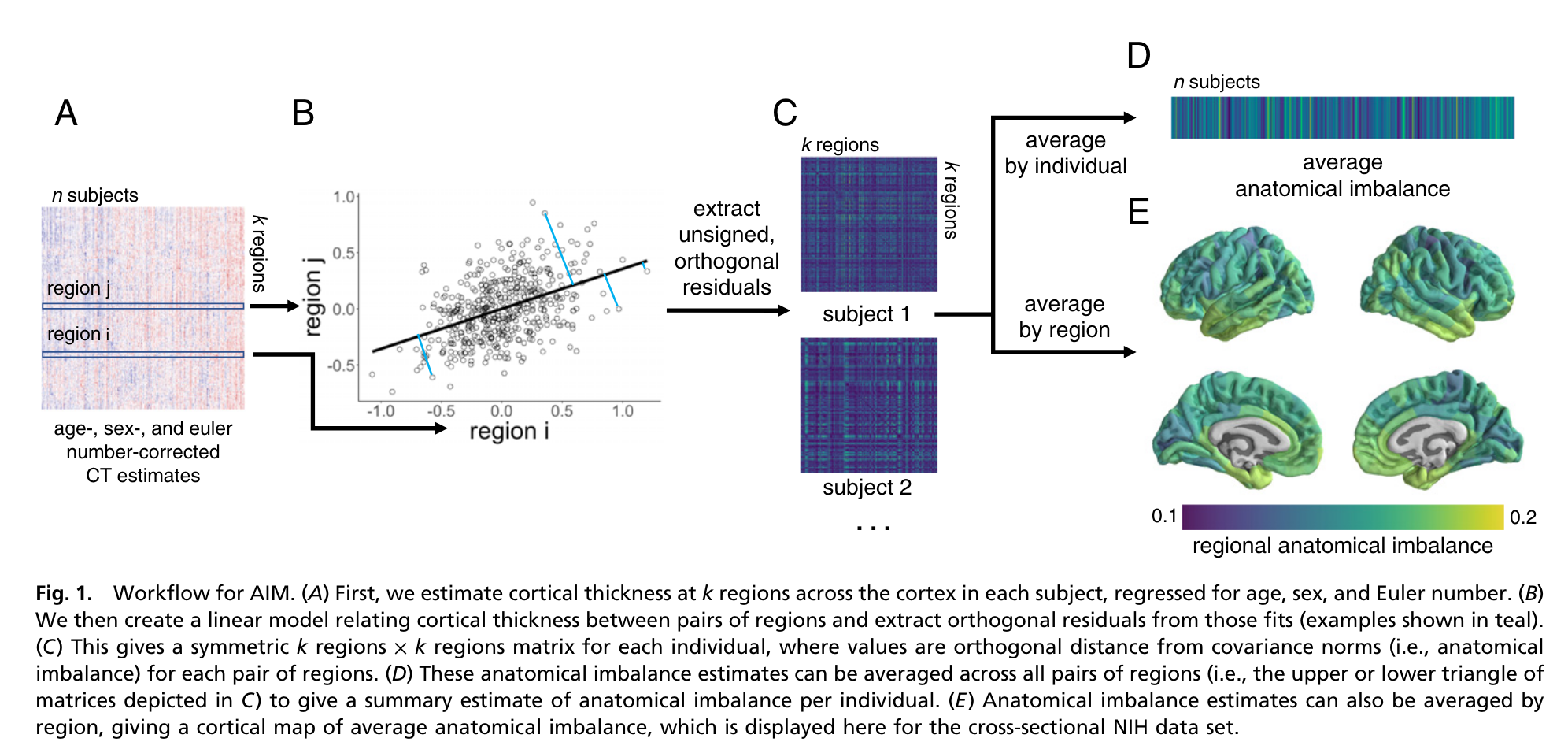
In this method, a higher residual value means a stronger deviation from the population norms. Note here that the regression between regions also uses what is called an orthogonal distance (ODR) or total least square regression. Contrary to an ordinary least square (OLS) regression where the error in the fitted values is assumed to only affect the outcome (i.e., y variable), an ODR assumes error in both the outcome and predictor. This is particularly relevant in our analysis as, since we are using grey matter measures for both predictor and error, we can’t assume that the values in one region are error-free. I talk more about the principles behind orthogonal regression in the tutorial.

Below are a few definitions that will be used throughout the module:

Definitions

Note that the original paper by Nadig et al. (2021)1 termed the method anatomical imbalance mapping. However, I believe that this method could be applied to other modalities rather than only anatomy. As such, I will refer to it by imbalance mapping throughout.

Orthogonal distance: Distance between the value of an individual to the ODR slope. Represents the “imbalance” (i.e., difference between an individual and the population).
Imbalance map: Matrix containing the orthogonal distances of one individual, for each pair of region.
Average imbalance by region: Average imbalance (i.e., orthogonal distance) for each brain region at the group-level
Average imbalance by person: Average imbalance (i.e., orthogonal distance) across regions at the individual-level
Average imbalance by person by region: Average imbalance (i.e., orthogonal distance) for each region at the individual-level

Data type

The imbalance mapping module currently only support tabular data (i.e., spreadsheets) in the form of a pandas.DataFrame where columns are the brain regions and the rows are the individual participants. sihnpy includes cortical thickness and volume for the 68 regions of the Desikan atlas 5 for 306 PREVENT-AD participants who had FreeSurfer-processed T1w imaging available.

Note that sihnpy won’t check if you have duplicates in your data. It will assume each row is unique. This is important as it can strongly influence your orthogonal distances.

Use cases and limitations

Imbalance mapping is quite recent, so it is difficult to determine what are the conditions of use. Here are what I have so far

Have measurements for at least more than 2 brain regions
Have at least 30 participants (see limitations)
Assume that there are population norms for the covariance of two regions
Covariance between regions should respect orthogonal regression assumptions
- Both the predictor and outcome have an error component
- Error terms of the predictor and outcome are independent
- Error terms have means of 0 and constant variances
- Predictor and outcome are linearly related

The original work on imbalance mapping focused mainly on anatomical data (i.e., thickness and volume). However, this could theoretically be applied to many different types of data, neuroimaging or not, as long as the assumptions above are respected. Furthermore, one should be aware of the following limitations:

Strength	Limitations
o Easy-to-apply individual-level measure	x Despite the name “imbalance”, it is difficult to say if having more imbalance is better or worse (interpretation is difficult)
o Measurements can be obtained at the individual-level and at the group level	x Structural covariance analyses are subject to many limitations (detailed below table)
o Computationally inexpensive as the module relies mostly on fast vectorized `numpy` functions	x Hasn’t been tested with highly dimensional data such as voxel-wise

Warning

Structural covariance, which was the theoretical basis of imbalance mapping can be influenced by many factors and show considerable heterogeneity between sites.

Carmon et al. (2020)6 list factors that can influence results of structural covariance which includes: lower image resolution, different preprocessing software versions, combining multi-site data, using cortical thickness (over volume and surface area), having a small sample (< 30 for the Desikan atlas). These factors should be properly accounted for before running imbalance mapping. Furthermore, both Nadig et al. (2021)1 and Carmon et al. (2020)6 correct for age and sex. As such, it is unclear how these factors impact imbalance mapping.

The data included in sihnpy does not correct for any of the above. This is done on purpose to let users explore the data on their own and I do not want to impose any of these choices on the user. Furthermore, certain information (like age) is not available in the PREVENT-AD Open Dataset.

Furthermore, sihnpy does not verify that the ODR assumptions are respected. This was mostly because I wasn’t exactly sure how to test them and as both Nadig et al. (2021) and most packages using ORD do not provide a way to check for these assumptions. Any input on this matter would be greatly appreciated; just open an issue. Depending on the request for this, I may also spend more time to figure it out.

Logistical considerations

The imbalance mapping module was developped and tested using PREVENT-AD data shipped in sihnpy. The code on this data (1 DataFrame; 306 rows and 68 columns) runs entirely in less than 10 seconds. As the functions for the ODR and the imbalance mapping were entirely implemented in sihnpy using the fast, vectorized pandas and numpy, the operations should normally always run fast. However, this wasn’t tests in much larger datasets or datasets with much higher dimensionality (e.g., voxel-level data).

Note also that depending on the exporting option chosen, sihnpy will output individual-level matrices of orthogonal distances. Depending on the number of regions and the number of participants, these matrices can become heavy in terms of storage. Keep in mind if using highly dimensional data.

References

Here are the papers cited throughout this section:

1(1,2,3,4,5): Nadig A, Seidlitz J, McDermott CL, Liu S, Bethlehem R, Moore TM, Mallard TT, Clasen LS, Blumenthal JD, Lalonde F, Gur RC, Gur RE, Bullmore ET, Satterthwaite TD, Raznahan A. Morphological integration of the human brain across adolescence and adulthood. Proc Natl Acad Sci U S A. 2021 Apr 6;118(14):e2023860118. doi: 10.1073/pnas.2023860118. PMID: 33811142; PMCID: PMC8040585.
2: Raznahan A, Lerch JP, Lee N, Greenstein D, Wallace GL, Stockman M, Clasen L, Shaw PW, Giedd JN. Patterns of coordinated anatomical change in human cortical development: a longitudinal neuroimaging study of maturational coupling. Neuron. 2011 Dec 8;72(5):873-84. doi: 10.1016/j.neuron.2011.09.028. PMID: 22153381; PMCID: PMC4870892.
3: Váša F, Seidlitz J, Romero-Garcia R, Whitaker KJ, Rosenthal G, Vértes PE, Shinn M, Alexander-Bloch A, Fonagy P, Dolan RJ, Jones PB, Goodyer IM; NSPN consortium; Sporns O, Bullmore ET. Adolescent Tuning of Association Cortex in Human Structural Brain Networks. Cereb Cortex. 2018 Jan 1;28(1):281-294. doi: 10.1093/cercor/bhx249. PMID: 29088339; PMCID: PMC5903415.
4: DuPre E, Spreng RN. Structural covariance networks across the life span, from 6 to 94 years of age. Netw Neurosci. 2017 Oct 1;1(3):302-323. doi: 10.1162/NETN_a_00016. PMID: 29855624; PMCID: PMC5874135.
5: Desikan RS, Ségonne F, Fischl B, Quinn BT, Dickerson BC, Blacker D, Buckner RL, Dale AM, Maguire RP, Hyman BT, Albert MS, Killiany RJ. An automated labeling system for subdividing the human cerebral cortex on MRI scans into gyral based regions of interest. Neuroimage. 2006 Jul 1;31(3):968-80. doi: 10.1016/j.neuroimage.2006.01.021. Epub 2006 Mar 10. PMID: 16530430.
6(1,2): Carmon J, Heege J, Necus JH, Owen TW, Pipa G, Kaiser M, Taylor PN, Wang Y. Reliability and comparability of human brain structural covariance networks. Neuroimage. 2020 Oct 15;220:117104. doi: 10.1016/j.neuroimage.2020.117104. Epub 2020 Jul 2. PMID: 32621973.